Multilabel classification is a common task in machine learning and Natural Language Processing (NLP). We approach it by training a model that can apply one or more labels to each new example that it sees. Since the model will output a probability for each of the labels, one of the parameters we can tweak to improve its performance (for example measured in micro f1) is the threshold probability at which a label is applied.
The most naive approach to this problem is to apply a label when the probability is >0.5, but this threshold can be higher (or lower). We can also decide to use a separate threshold for each label, and selecting the right one for each label is an optimization problem in its own right.
This blog post is about how we sped up an implementation of an algorithm to solve this problem, and reduced its run time from 31 days to just five minutes.
The approach we followed is the one proposed by Pillar, et al. (2013) in their research paper “Threshold optimization for multi label classifiers”. The proposed algorithm for solving this optimization problem can be seen in the pseudo code-below:.
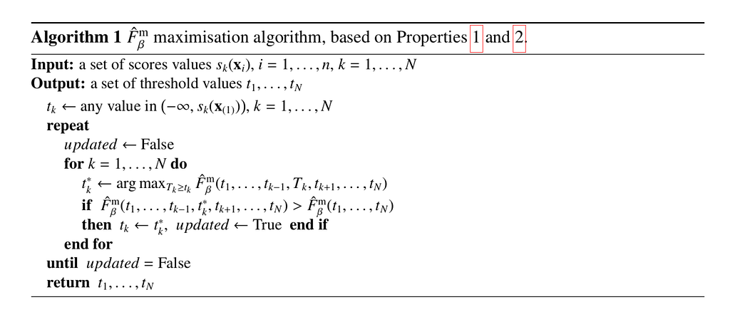
This algorithm effectively attends one label at a time and tries all possible thresholds for that label to find the threshold with the best micro f1. It does that iteratively (since a decision for one threshold might influence another) until no better threshold can be found for any label. Below is a naive implementation in python.
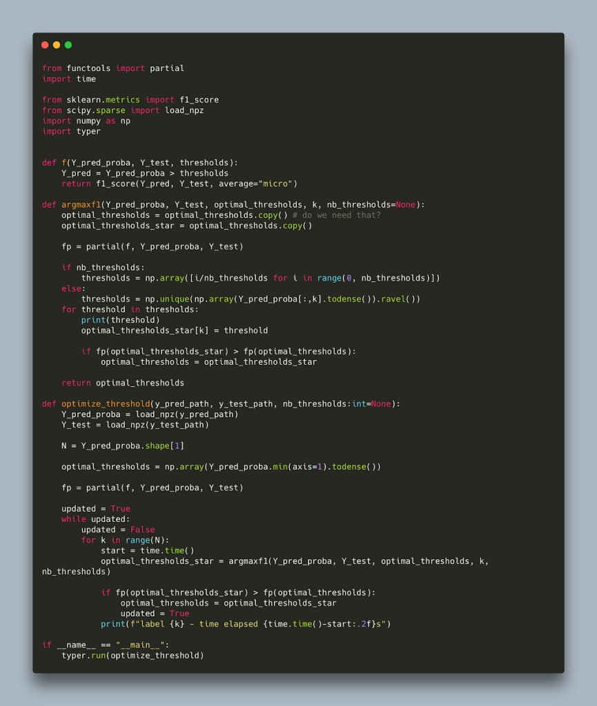
The code closely follows the pseudo code in the paper with the addition of the nb-thresholds parameter to limit the number of thresholds to scan thereby decoupling the run time from the dataset size used. Running this algorithm on two randomly sparse matrices takes 30s per label. This makes it prohibitively expensive for large label spaces, for example: assuming we need three iterations for the algorithm to converge and we are working with 30k labels it would take 30s x 30,000 x 3 ~ 31 days!
Since we can’t usually wait 31 days just to decide which labels to apply after prediction, we needed to find a way to speed up this algorithm. The rest of this blog post focuses on just this problem. We’ll be using a tool called line_profiler to inspect the slow moving parts of the algorithm and work towards making it faster.
Line profiler was brought to my attention from the excellent book High performance python by Ian Ozvald and Micha Gorelick, which I highly recommend if you want to speed up your python code. All we need to do is install the line profiler pip install liner_profiler and add the @profile decorator in the functions we want to profile. Running our algorithm with it produces the following output:
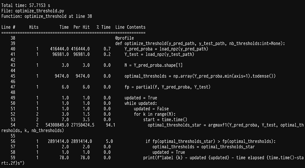
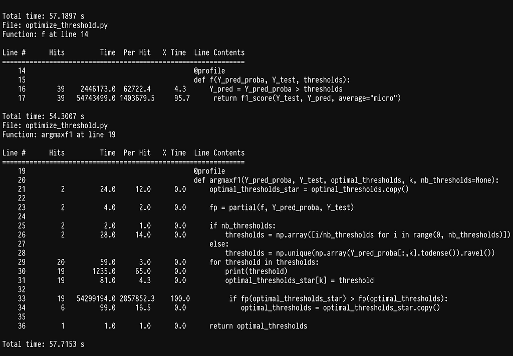
As we can see most of the time is being spent inside the sklearn function f1_score. If we go ahead and profile it by adding the @profile decorator in the argmax function we get:

As it turns out, half of the time is being spent on checking that the data being passed are correct (see line 1547). This is super helpful in most cases, as it will throw an error if the data or flags do not make sense, but quite inefficient in our case, as we constantly pass the same data. Since we cannot disable this behavior we can simply write our own f1_score function.
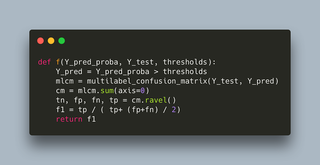
This reduces runtime to 17s per label which is half our first attempt but still quite slow. If we profile again we get

In line 17, we see that we seem to have shifted the weight to sklearn’s multilabel_confusion_matrix. Let’s profile the multilabel_confusion_matrix function by adding the @profile decorator in the internal of sklearn’s code. You can find the location where site-packages are installed by running python -m site. The multilabel confusion matrix leaves in _classification.py inside metrics, full path sklearn/metrics/_classification.py.

We run into the same problem of spending most of the time checking that the y variables are correct, see line 483. Once more we can write our own implementation to avoid the checks.
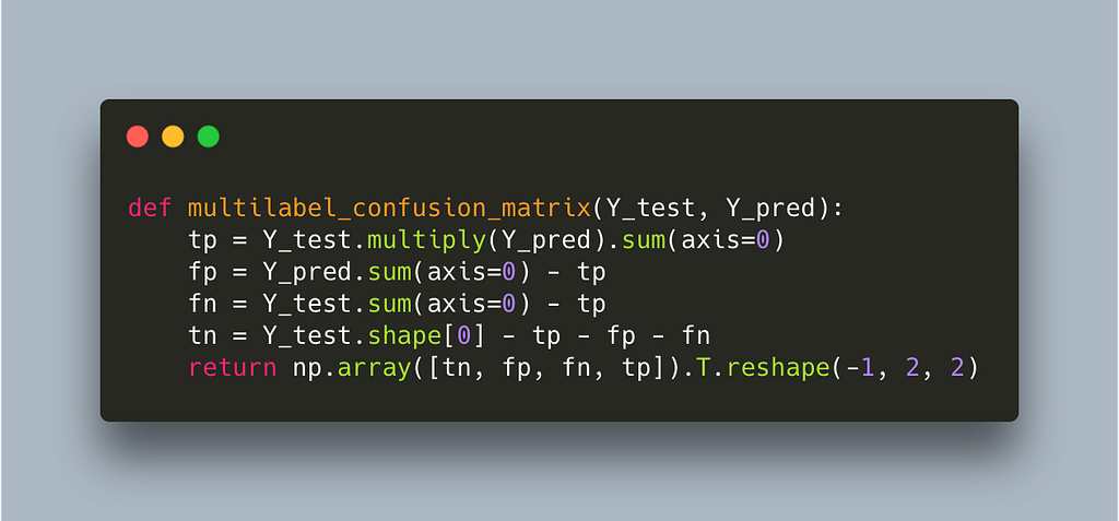
https://github.com/nsorros/threshold%5Foptimizer/commit/7df2d45cda077662f2846a80edbce0c8a0383161
Using our own multilabel confusion matrix further reduces the time to 3s which is a 10x improvement so far. Let’s see what’s slowing us down now.
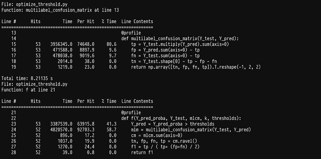
We can see that most of the time is being spent in the element-wise multiplication of two large sparse matrices. There is an inefficiency here which is not obvious at first glance: the multilabel confusion matrix recalculates a confusion matrix for each label even though we only alter the threshold for one label. A much more efficient way would be to calculate the multilabel confusion matrix outside this function and ultimately the for loop across labels and only change the entry for the label we explore. This requires us to calculate only one confusion matrix and I think at this point it is obvious that we are better off writing our own implementation.
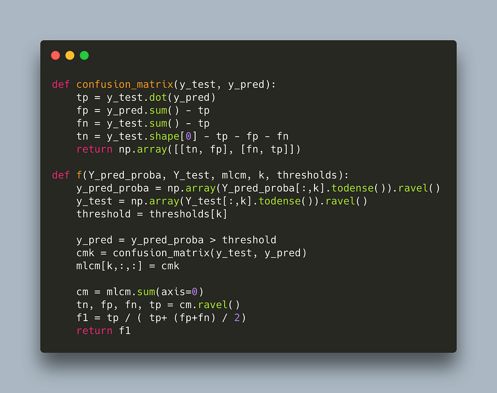
https://github.com/nsorros/threshold%5Foptimizer/commit/7df2d45cda077662f2846a80edbce0c8a0383161
At this point our algorithm takes 0.46s per label which is a 65x speedup. In fact the whole optimization can finish in 5 hours which is acceptable. But, can we do better?
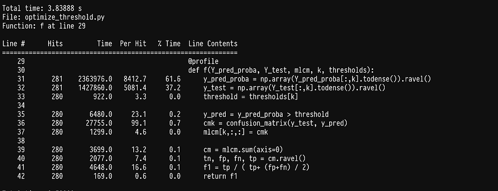
A seemingly simple operation of choosing the relevant column, lines 31–32, seems to add up to a significant cost when running multiple times. Since those columns remain the same for the duration of trying different thresholds for one label inside argmax, we can easily improve by picking those columns before calling argmaxf1 and passing them in.
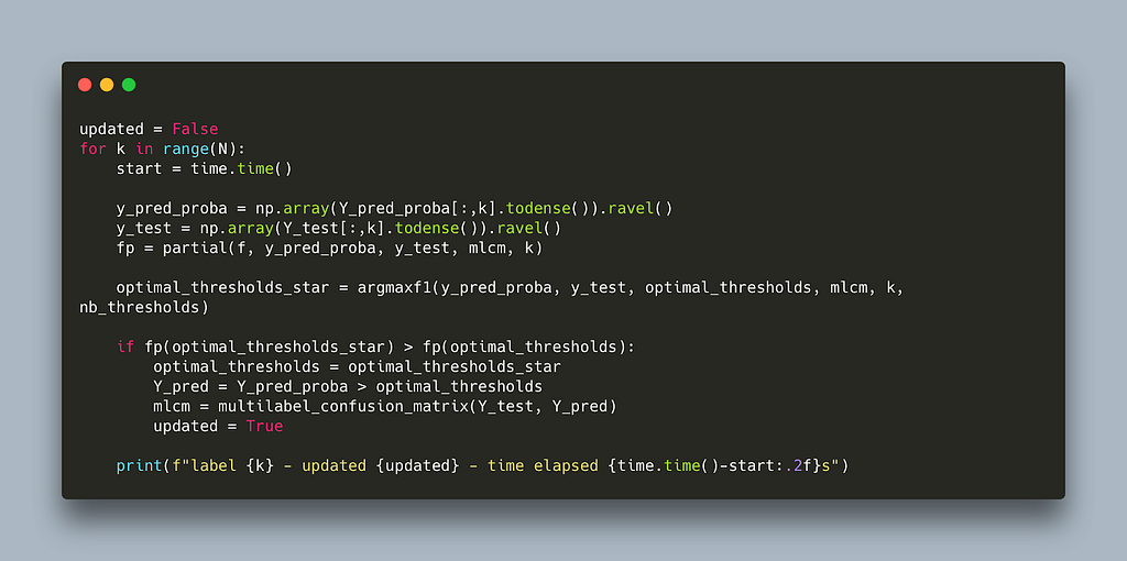
https://github.com/nsorros/threshold%5Foptimizer/commit/d8a2b8755bc244c22e8a1758b06ab597c6fff2db
This change reduces the time to 0.17s per label which is a 176x speedup. This is beginning to be fast 💨 but let’s see if we can push it further.
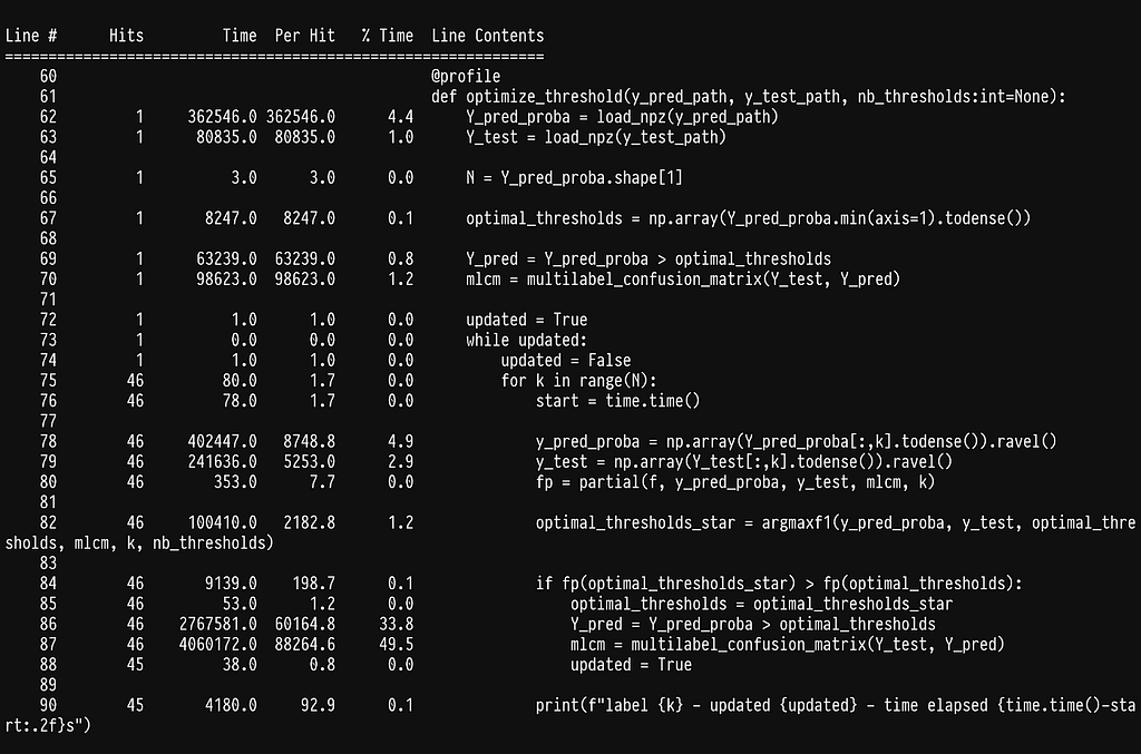
Every time we update the thresholds we recalculate the multilabel confusion matrix, line 87, and this is quite expensive. We can employ the same trick we did earlier inside f where we calculate only the confusion matrix that changes.
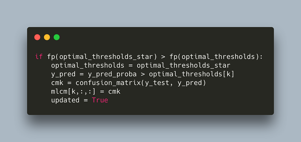
https://github.com/nsorros/threshold%5Foptimizer/commit/06cb7a127366aa9844b010e666f5e99190987a64
This takes us down to 0.02s per label which offers another 10x speedup for a total of 1500x. We could call it a day but let’s see if there is any other easy win.
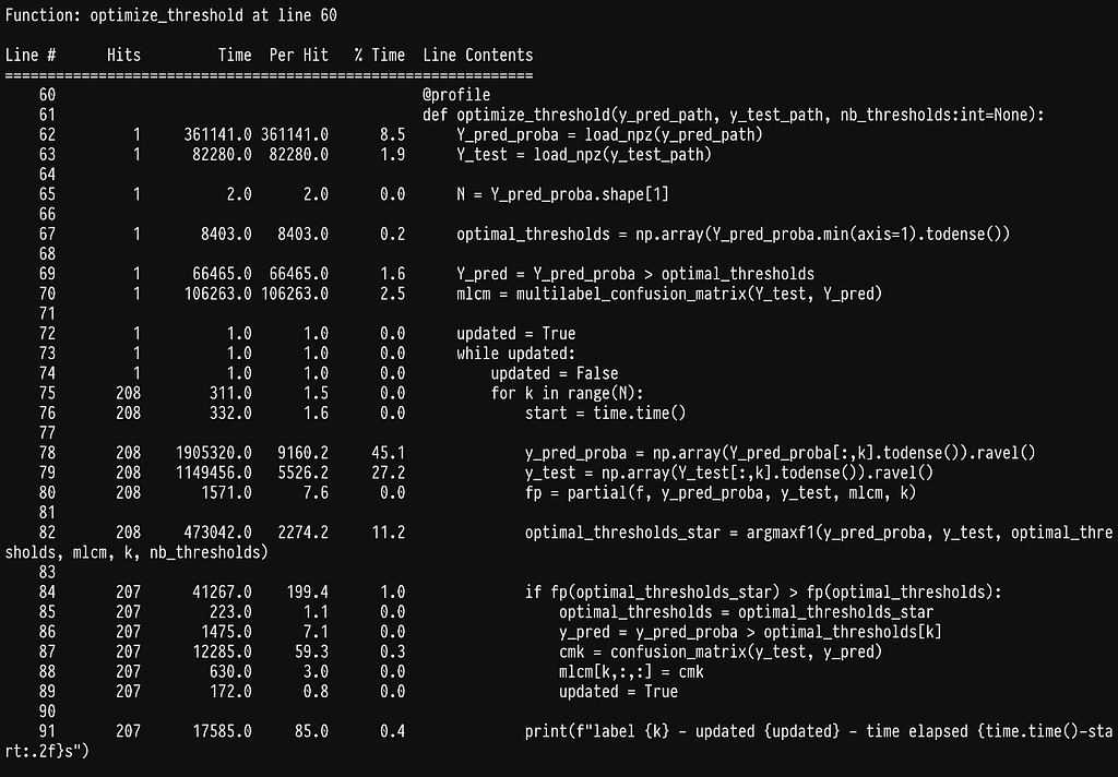
We can see that a lot of time is being spent on selecting a column of a sparse matrix, lines 78–79. As it turns out these matrices are in CSR format which is quite efficient for a lot of common data science operations but not for selecting columns
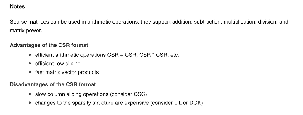
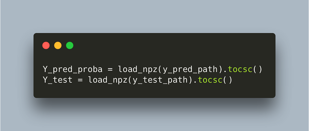
Fortunately for us we can simply convert to CSC in load time and not have to worry about it moving on.
https://github.com/nsorros/threshold%5Foptimizer/commit/06cb7a127366aa9844b010e666f5e99190987a64
This switch makes the algorithm run on 0.003s per label which gives us a 10k final speedup. The whole algorithm will take approximately 5 minutes for 30k labels and a few hours for millions of labels which is super fast for the problem at hand. We can stop here but it’s worth saying that we have reached a limit of diminishing returns if we continue. Most of the time is being spent on highly optimized functions in numpy and scipy and even if we write our own and compile them with numba we will not manage to go any faster.
This blog has walked through the problem of how to optimize a naive implementation of an algorithm. Whilst the starting problem is not relevant to everyone, the techniques which I have used to speed up the implementation are super powerful, and can be applied to any problem.
You can find the whole code in this repository https://github.com/nsorros/threshold%5Foptimizer and you can also follow the first 8 commits which introduce these changes.
Making an optimisation algorithm 10k times faster 🏎 was originally published in MantisNLP on Medium, where people are continuing the conversation by highlighting and responding to this story.